
| 일 | 월 | 화 | 수 | 목 | 금 | 토 |
|---|---|---|---|---|---|---|
| 1 | ||||||
| 2 | 3 | 4 | 5 | 6 | 7 | 8 |
| 9 | 10 | 11 | 12 | 13 | 14 | 15 |
| 16 | 17 | 18 | 19 | 20 | 21 | 22 |
| 23 | 24 | 25 | 26 | 27 | 28 | 29 |
| 30 |
- Heap
- 빅데이터 지식
- Data Engineer
- 데이터 분석가
- hash
- data
- Study
- BST
- 뉴욕 화장실
- Data Structure
- Computer Science
- 데이터 엔지니어
- algorithm
- Data Analyst
- binary search tree
- 빅데이터
- Computer Organization
- Preparing for the Google Cloud Professional Data Engineer Exam
- priority queue
- dataStructure
- 화장실 지도
- exam
- Newyork
- HEAPS
- Algorithms
- Restroom
- data scientist
- 빅데이터 커리어 가이드북
- Linked List
- Binary Tree
- Today
- Total
Jaegool_'s log
데이터분석 종합반 3주차[스파르타 코딩]<Data Visualization> 본문
데이터분석 종합반 3주차[스파르타 코딩]<Data Visualization>
Jaegool 2022. 6. 18. 21:48https://teamsparta.notion.site/3-cdea49d6bc514763b80d5508ca92e4ca
[스파르타코딩클럽] 데이터분석 종합반 - 3주차
매 주차 강의자료 시작에 PDF파일을 올려두었어요!
teamsparta.notion.site
<how to get some data>
import pandas as pd
url = 'https://raw.githubusercontent.com/justmarkham/DAT8/master/data/drinks.csv'
drink_df = pd.read_csv(url, ',')
<Access to several columns(다수의 열에 접근하기)>

- nameOfDataFrame[LIST]
ex) drink_df[['beer_servings','wine_servings']]
<Using conditional logic(조건부 로직 사용하기)>

ex) drink_df[drink_df.continent=='EU'].head(20)
<import matplotlib.pyplot & seaborn>
import matplotlib.pyplot as plt
import seaborn as sns
<plt.pie>

pie_labels = drink_df['continent'].value_counts().index.tolist()
pie_values = drink_df['continent'].value_counts().values.tolist()
print(pie_labels)
print(pie_values)
['AF', 'EU', 'AS', 'ETC', 'OC', 'SA']
[53, 45, 44, 23, 16, 12]plt.pie(pie_values, labels=pie_labels, autopct='%.02f%%')
plt.title('Percentage of each continent')
plt.show()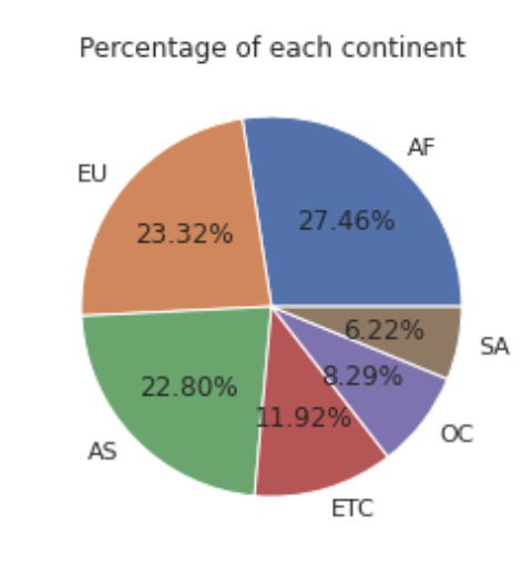
<Using Group By>

<Charts>
# barchart를 이용해 species 표현
df['species'].value_counts().plot(kind='bar')

# seaborn을 이용한 barchart
# EX 1)
sns.barplot(df['species'], df['sepal width (cm)'], ci=None)

# EX 2)
sns.barplot(x='confirmed', y='city', data=case[case['province']=='Daegu'], ci=None).set(xlabel='Confirmed', ylabel='Districts', title='Case in Daegu')
sns.barplot(x=열의 이름, y=열의 이름, data=데이터프레임, ci=None)
.set(xlabel='x축에 대한 레이블', ylabel='y축에 대한 레이블', title='차트의 타이틀')
df['petal width (cm)'].plot(kind='hist')
plt.title('Iris Petal Width', fontsize=14, y=1.01)
plt.ylabel('Value')
plt.xlabel('Width')
그 외에도 'line', 'bar', 'barh', 'box', 'kde', 'density', 'area', 'pie'와 같은 값들이 가능합니다.
이에 대해선 아래의 Pandas Series의 공식 문서에서 확인할 수 있습니다.
https://pandas.pydata.org/pandas-docs/version/0.24.2/reference/api/pandas.Series.plot.html
pandas.Series.plot — pandas 0.24.2 documentation
Parameters: data : Series kind : str ‘line’ : line plot (default) ‘bar’ : vertical bar plot ‘barh’ : horizontal bar plot ‘hist’ : histogram ‘box’ : boxplot ‘kde’ : Kernel Density Estimation plot ‘density’ : same as ‘kde’ ‘
pandas.pydata.org
#seaborn을 이용한 산점도
sns.pairplot(df, hue="species")
<Visualization of Series>
NameOfSeries.plot()
# EX)
plt.rcParams['figure.figsize'] = (15, 5) # 그래프 비율 조정
daily_count.plot()
plt.title('Number of Daily Confirmed Patients')
<Visualization of Map & HeatMap>
import folium
from folium import plugins

seoul = folium.Map(location=[37.55, 126.98], zoom_start=12)
seoul

# 서울을 표시하기 위한 변수는 seoul
# Stamen Terrain 옵션 선택.
seoul = folium.Map(location=[37.55, 126.98], zoom_start=12, tiles='Stamen Terrain')

latitude, longitude = 35.9078, 127.7669 # 대한민국의 좌표
S_korea = folium.Map(location = [latitude, longitude], zoom_start = 8)
S_korea

# HeatMap 추가
# - **폴리움객체.add_child(plugins.HeatMap(zip(위도, 경도, 정도), radius=18))**
S_korea.add_child(plugins.HeatMap(zip(local_infected['latitude'],
                                      local_infected['longitude'],
                                      local_infected['confirmed']), radius=18))

# RecursionError: maximum recursion depth exceeded
# - Because of object type, latitude & longitude should be 'float' type.
# https://mskim8717.tistory.com/79 - 참고하기

local_infected['latitude'] = local_infected['latitude'].astype('float')
local_infected['longitude'] = local_infected['longitude'].astype('float')

S_korea.add_child(plugins.HeatMap(zip(local_infected['latitude'],
                                      local_infected['longitude'],
                                      local_infected['confirmed']), radius=18))
# **만약 True, False 각각 그룹에 대한 확진자 수가 궁금하다면 어떻게 하면 좋을까요?**
# - pivot_table(index = ['그룹핑하고 싶은 열의 이름'], aggfunc = '그룹핑 후에 수행할 연산')
group_cases = case.pivot_table(index = ['group'], aggfunc = 'sum').reset_index()
group_cases
# replace
group_cases = group_cases.replace({True: 'Locally infected', False: 'From outside'})
group_cases
# 데이터를 시각화 할 때는 데이터를 자세히 살펴봐야 합니다.
# 시각화를 할 때 오류가 나는 대부분이 경우가 데이터에 결측값 또는 의미없는 값 등이 있는 경우가 많습니다.
# group이 True라고 하더라도 위도, 경도가 누락이 된 경우가 있는지 확인해봅시다.
<HW>

plt.figure(figsize=(5, 5))
sns.heatmap(df_data.corr(), annot=True)
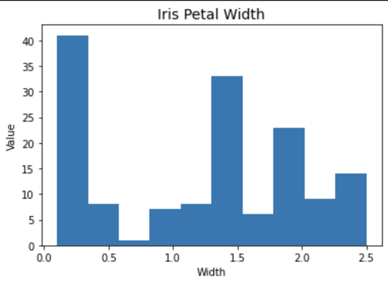
df['petal width (cm)'].plot(kind='hist')
plt.title('Iris Petal Width', fontsize=14)
plt.ylabel('Value')
plt.xlabel('Width')
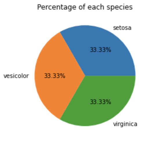
pie_labels = df['species'].value_counts().index.tolist()
pie_values = df['species'].value_counts().values.tolist()
print(pie_labels)
print(pie_values)

plt.pie(pie_values, labels=pie_labels, autopct='%.02f%%')
plt.title('Percentage of each species')
plt.show()
sns.pairplot(df, hue='species')'Development Log > Data Analytics' 카테고리의 다른 글
| 데이터분석 종합반 5주차[스파르타 코딩]<고객 행동 예측, 고객 행동 예측> (0) | 2022.06.28 |
|---|---|
| 데이터분석 종합반 4주차[스파르타 코딩]<LinearRegression, 자전거 수요 예측 준비 단계> (0) | 2022.06.25 |
| 데이터분석 종합반 2주차[스파르타 코딩]<데이터 시각화, 워드클라우드, 벡터화, 머신러닝> (0) | 2022.06.12 |
| Data analysis 1st week [SpartaCoding] <Kaggle, Colab, BeautifulSoup4> (0) | 2022.06.01 |


